Table of Contents:

1. Types of Geospatial Data
2. Vector Data Formats
3. Raster Data Formats
4. Practical Example with QGIS

Types of Geospatial Data

There are primarily two categories of geospatial data: vector data and raster data. Vector data retains a tabular format, while raster data resembles colorful images composed of three color channels: red, green, and blue.

Focusing on vector data, we can categorize it into three main types: point data, line data, and polygon data.

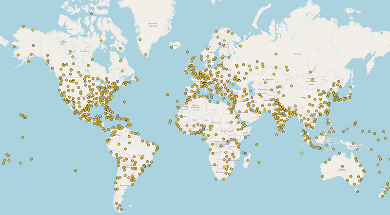
Point data represents the simplest form, defined by a pair of coordinates—latitude and longitude. Examples include cities, restaurants, and shopping centers. The image above illustrates point data, showcasing the locations of airports worldwide, sourced from Natural Earth Data, one of many accessible data resources.

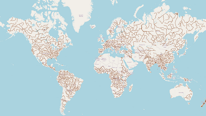
Next, we explore line data, which consists of a line defined by a starting and an ending point. Typical examples include streets, train routes, and rivers, as depicted below.

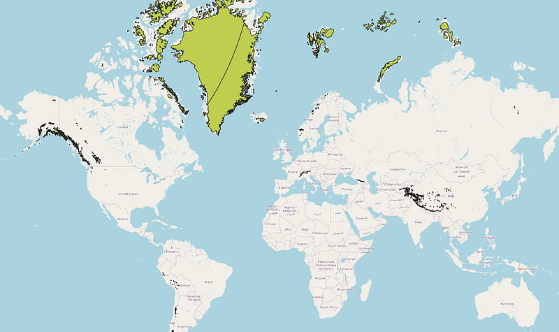
Lastly, polygon data is formed by a series of interconnected points that create a closed shape. A simple way to visualize this data type is by considering the boundaries of countries. Below, you will find an overview of glaciers and recently deglaciated regions.

Following our discussion on vector data, we turn our attention to raster data, which I find particularly fascinating. While raster data may resemble images due to their pixel matrix structure, each pixel represents a unique geographic area, with its value describing specific characteristics of the terrain.

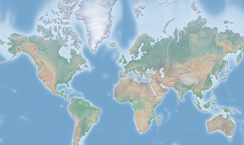
As shown in the visualization, raster data can convey more comprehensive information about real-world surfaces compared to vector data. Examples of raster data include satellite images and aerial photographs, which are vital for disaster monitoring and accelerating rescue efforts. Thus, this data not only provides valuable insights for businesses but can also save lives, particularly when deep learning models are trained to identify specific objects in satellite imagery.

Vector Data Formats

Understanding file formats is crucial when working with geospatial data. The most prevalent format for vector data is the Shapefile, commonly found in numerous free, open-source datasets. When you download vector data, it typically comes in a zip file containing three essential files:

• .shp: This is the primary file containing the geometry necessary for plotting points, lines, and polygons on the map.
• .dbf: This database file holds attribute data, which includes non-geospatial information that contextualizes the geospatial data, such as names of cities, rivers, streets, and countries.
• .shx: This file provides the positional index of the feature geometry, linking attributes to geometry.

Another frequently used format is GeoJSON (Geographic JavaScript Object Notation), which is designed for web-based mapping and comprises two files: .geojson and .json.

Raster Data Formats

Raster data also has a standard format known as GeoTIFF. Similar to Shapefiles, it includes three files: .tif, .tiff, and .ovr. While GeoTIFF and Shapefiles may come with additional files, these are not mandatory.

Other format alternatives include ERDAS Imagine (.img) and IDRISI Raster (.rst, .rdc). That’s all for the formats!

Practical Example with QGIS

QGIS is the open-source software we'll use to visualize geospatial data. If you haven’t installed QGIS yet, you can download it from here. Once installed, you will see a window that looks like this:

To begin, add a background map to your map window. The most common method is to utilize OpenStreetMap, which offers the largest free and editable geographic database, continually updated by a dedicated team of volunteers. The steps to add it are straightforward:

1. Click the arrow next to “XYZ Tiles” in the Panels.
2. Double-click on OpenStreetMap.

And there you have it! We have successfully imported OSM data into our QGIS project. Next, we can drag the geographic data you wish to analyze into the Layers Panel. For instance, let’s import the airport data from Natural Earth Data, as previously mentioned.

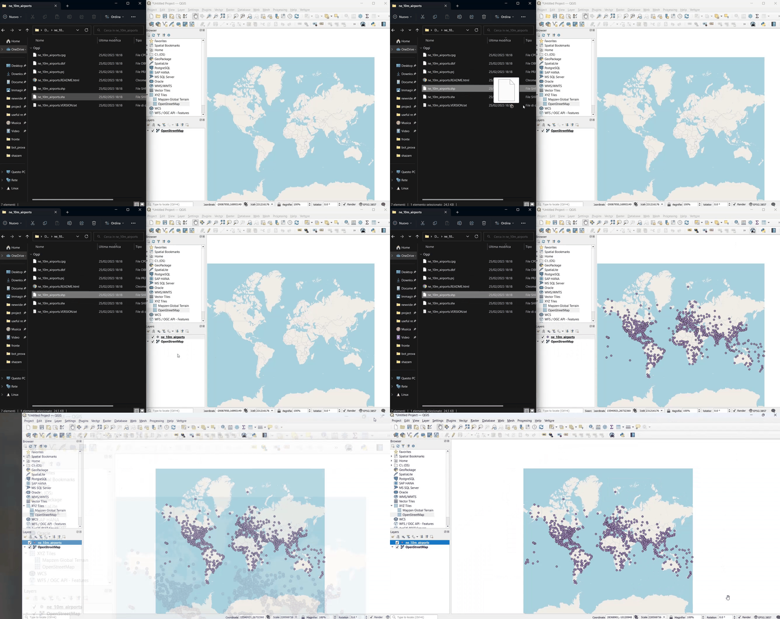
We can also review the data’s information and adjust the color of the points:

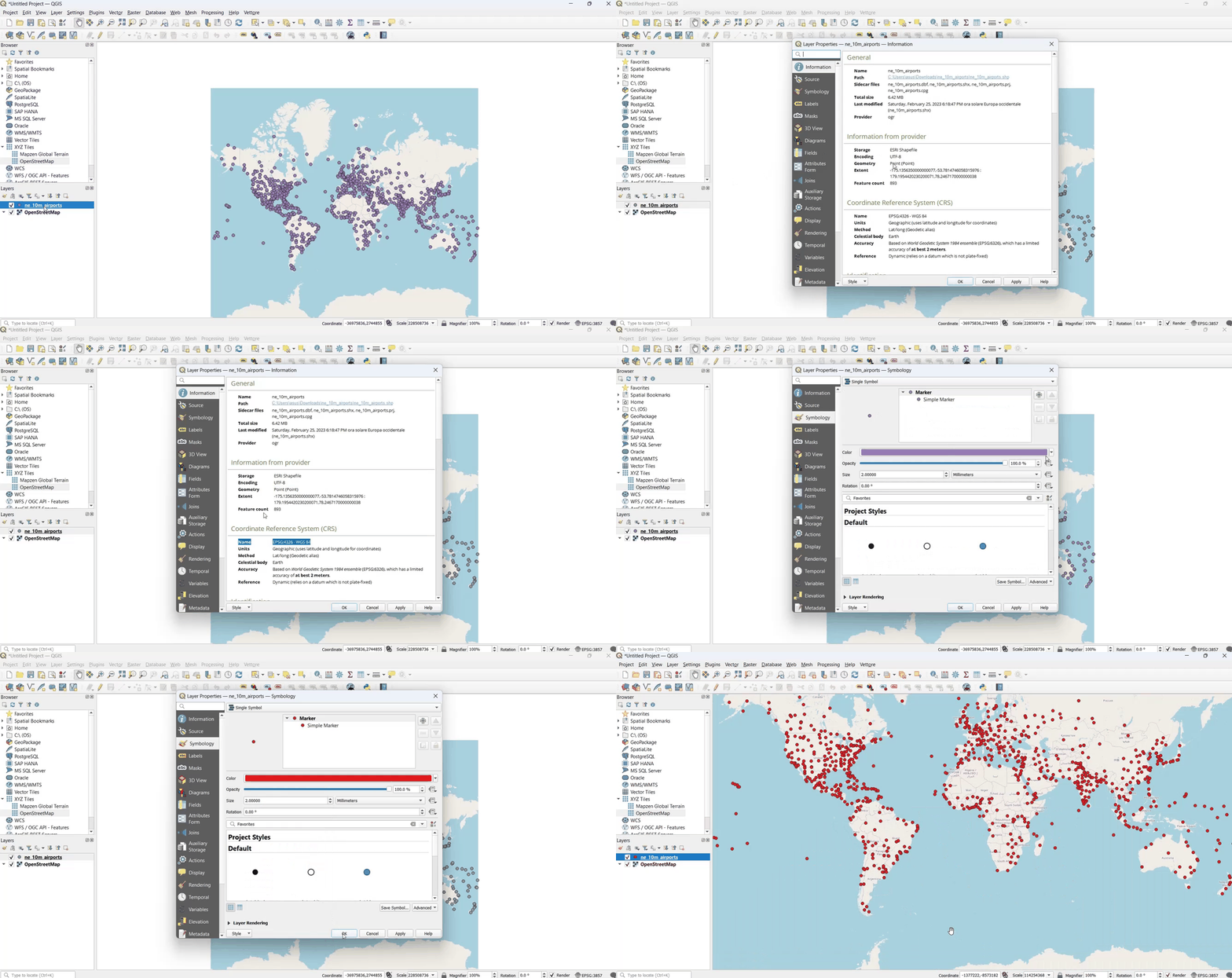
The Information section provides an overview of the data type (point data) and the coordinate reference system (CRS), which is essential for accurately translating locations on Earth, characterized by an irregular spheroid shape, into a 2D map. You'll notice that the CRS in use doesn't match that of QGIS and requires adjustment.

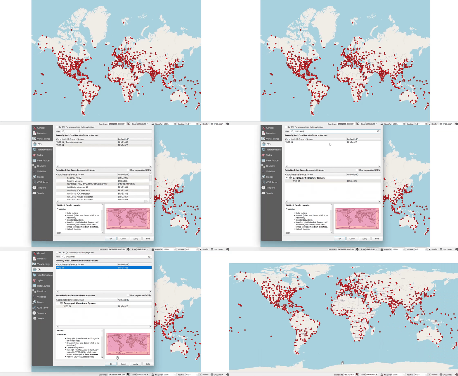
Now that we've corrected the error, we can breathe a sigh of relief.

Final Thoughts

That wraps up this quick and concise tutorial, introducing you to the captivating world of geospatial data analysis. I chose to use QGIS for this tutorial to provide straightforward examples of geospatial data. This is merely the beginning. In upcoming articles, I will delve into additional applications utilizing Python libraries. If you’re keen to explore further and find free GIS data sources, check here.

Useful Resources:

• Getting Started with Geospatial Works by Dhrumil Patel
• GIS Documentation
• Analyze Geospatial Data in Python: GeoPandas and Shapely
• Introduction to Geospatial Concepts