A Brief Overview of the loc Method

The loc method in Pandas allows users to select specific rows or columns from a DataFrame based on defined conditions. You can pass various inputs to loc; for instance, if you want to select a slice of a DataFrame using its index, you can apply the same syntax as list slicing in Python, such as: [start:stop]. However, for this discussion, we will focus on utilizing loc with conditional statements. This is somewhat akin to the WHERE clause in SQL, which filters data.

In general, using loc in this context would look like this:

df.loc[df["column"] == "condition"]

This expression returns a subset of the data where the column matches the specified condition.

Now let's delve into practical examples of using the loc method for exploratory data analysis.

Section 1.1: Analyzing University Attendance with loc

Which universities only offer in-person attendance?

To determine this, we can use loc to filter the relevant data for analysis. If the data were clean, one might think to simply employ a groupby operation on the column to count institutions offering in-person attendance. In Pandas, this could be expressed as:

df.groupby("Distance / In-Person")["Institution"].count()

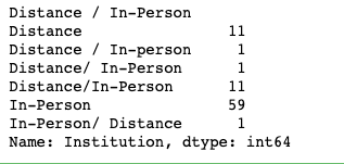
However, the values in the “Distance / In-Person” column are not well-organized. There are whitespace issues, and some universities provide both distance and in-person attendance in an inconsistent format.

To begin cleaning this data, we should rename the column to eliminate any spaces or special characters:

df = df.rename(columns={"Distance / In-Person": "distance_or_in_person"})

We can confirm this change by checking the DataFrame columns:

df.columns

Next, we can utilize the value_counts method to count unique values in the target column, which can be done as follows:

df["distance_or_in_person"].value_counts()

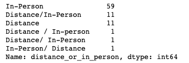
To further refine this column, we will group institutions that offer both types of attendance into a single category. Using loc, we can filter the DataFrame and assign a new value “Both” to the relevant entries:

df.loc[

~df["distance_or_in_person"].isin(["In-Person", "Distance"]),

"distance_or_in_person"

] = "Both"

This command selects rows where the distance_or_in_person column does not equal “In-Person” or “Distance”, and updates them to “Both”. Let’s verify the changes by examining the DataFrame again:

df.head()

Now, the updated column contains only three distinct values. We can use value_counts once again to answer our initial question:

df["distance_or_in_person"].value_counts()

From the cleaned dataset, we find that 59 universities offer only in-person attendance.

To identify the specific institutions that provide in-person options, we can filter the DataFrame with loc and convert the results to a list:

df.loc[df["distance_or_in_person"] == "In-Person"]["Institution"].tolist()

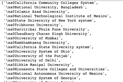
We now have a list of institutions, but it may contain special characters that need removing. The “xa0” symbol in Python signifies a non-breaking space, which we can eliminate using the strip method:

df.loc[df["distance_or_in_person"] == "In-Person"]["Institution"].str.strip().tolist()

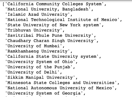
Now we have our final list of universities that exclusively offer in-person attendance!

Section 1.2: Year Range Analysis of Universities

What is the year range between the oldest and newest founded universities?

Next, let's employ loc and additional Pandas functions to analyze the year range of university foundations. We'll first examine the Founded column:

df["Founded"]

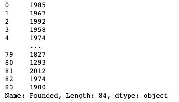
We see that this column contains year values. To facilitate comparisons, we can convert this column to a datetime type:

pd.to_datetime(df["Founded"])

However, doing so may result in a ParserError due to a string that doesn't fit the expected format. We can identify the problematic entry using loc:

df.loc[df["Founded"] == "1948 and 2014"]

It appears one university has two founding years listed. We can also filter based on the index of this row:

df.loc[9]

Depending on our analysis needs, we could either choose one year or create two separate entries for this institution. For simplicity, we will remove this row:

df.drop(9).head(10) # Remove the problematic row

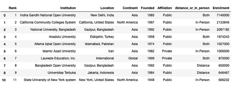
To make the drop permanent, we need to reassign the DataFrame:

df = df.drop(9)

Now, we can reattempt the datetime conversion:

pd.to_datetime(df["Founded"], errors="coerce")

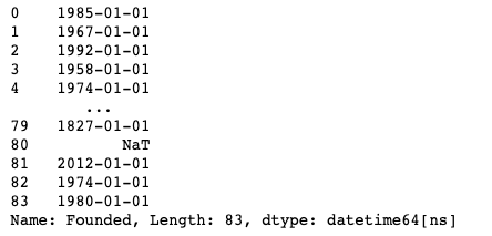
If any issues arise during conversion, they will be set to null due to the use of errors="coerce".

Next, we can create a new column for the datetime values:

df["founded_date"] = pd.to_datetime(df["Founded"], errors="coerce")

To discover the earliest founding date, we can employ the min method:

min(df["founded_date"])

To find the range of founding years between the oldest and newest universities, we can simply convert the Founded column to an integer type and subtract the min from the max:

df["Founded"] = df["Founded"].astype("int")

max(df["Founded"]) - min(df["Founded"])

This calculation yields a range of 719 years. While this approach is quick, it may not always be the best solution, especially when more intricate analysis is required. Properly cleaning and converting data to a datetime format has considerable advantages for thorough analyses.

The loc method is incredibly versatile, allowing you to filter, slice, and update your DataFrame to suit specific questions and challenges. Remember that data cleaning is an ongoing process that closely aligns with data exploration. I hope these examples of using loc will assist you in your future analyses.